JIT - a bit of look inside

The previous post about our JIT explained a bit from the 1000 km perspective how the tracing JIT would approach a language like Python.

I would like to step a bit inside and give a zoom to some of its features that are already working. While probably not the most innovative, I think it's very nice to look at the way we work with the JIT and what tools we use.

The main cool thing is that you can work on and try the JIT (including trying it on the Python interpreter!) without even generating a single bit of assembler. How? Let's start with something very simple. Let's take a simple interpreter for language X.

Language X has 3 opcodes: CO_INCREASE, CO_DECREASE and CO_JUMP_BACK_3. CO_INCREASE increase the accumulator by one, CO_DECREASE decrease it by one, CO_JUMP_BACK_3 jump 3 opcodes back, if the accumulator is smaller than 100 (this is only to maintain some halting conditions possible). The interpreter for language X looks like this::

    jitdriver = JitDriver(greens = ['i'], reds = ['res', 'a'])
    code = [CO_INCREASE, CO_INCREASE, CO_INCREASE,
            CO_JUMP_BACK_3, CO_INCREASE, CO_DECREASE]
            
    def add(res, a):
        return res + a

    def sub(res, a):
        return res - a

    def main_interpreter_loop(a):
        i = 0
        res = 0
        c = len(code)
        while i < c:
            jitdriver.jit_merge_point(res=res, i=i, a=a)
            elem = code[i]
            if elem == CO_INCREASE:
                res = add(res, a)
            elif elem == CO_DECREASE:
                res = sub(res, a)
            else:
                if res > 100:
                    pass
                else:
                    i = i - 3
                    jitdriver.can_enter_jit(res=res, i=i, a=a)
                    continue
            i = i + 1
        return res

All very simple code, expect the jitdriver hints, which instruct JIT how to behave (they are the equivalent of the ``add_to_position_key`` of last the blog post).

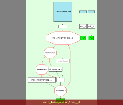
Let's look how this code is processed. This will also give a glance at how we work in this code. This particular piece can be found on a branch in pypy/jit/metainterp/test/test_loop.py and can be run with ./test_all.py jit/metainterp/test/test_loop.py -k test_example -s --view from pypy directory. The -s option lets you see the debugging output, while --view will show you some graphs. So, let's look at graphs in order:

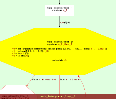
And the same picture with a bit of zoom for the first block:

This is the call graph of an interpreter loop, nothing magic so far. This is an intermediate representation of translation toolchain input. If you look around you can follow how the opcodes are dispatched (with a chain of ifs) and helpers called. Next graph is very boring, because it's a bit lower level representation of the same thing (you exit with q or escape btw :).

When we exit the graph viewer, we can see the trace generated by interpreting this graph with a given bytecode (variable code in paste above). It's something like:

        [compiler] ENTER
        [runner:cpu]    call__4 [(''), * GCREF hidden, 0] -> 0
        [runner:cpu]    int_eq [0, 0] -> True
        [runner:cpu]    int_add [9, 1] -> 10
        [runner:cpu]    int_add [0, 1] -> 1
        [runner:cpu]    int_lt [1, 6] -> True
        [runner:cpu]    call__4 [(''), * GCREF hidden, 1] -> 0
        [runner:cpu]    int_eq [0, 0] -> True
        [runner:cpu]    int_add [10, 1] -> 11
        [runner:cpu]    int_add [1, 1] -> 2
        [runner:cpu]    int_lt [2, 6] -> True
        [runner:cpu]    call__4 [(''), * GCREF hidden, 2] -> 0
        [runner:cpu]    int_eq [0, 0] -> True
        [runner:cpu]    int_add [11, 1] -> 12
        [runner:cpu]    int_add [2, 1] -> 3
        [runner:cpu]    int_lt [3, 6] -> True
        [runner:cpu]    call__4 [(''), * GCREF hidden, 3] -> 1
        [runner:cpu]    int_eq [1, 0] -> False
        [runner:cpu]    int_eq [1, 2] -> False
        [runner:cpu]    int_gt [12, 100] -> False
        [runner:cpu]    int_sub [3, 3] -> 0
        [compiler] LEAVE

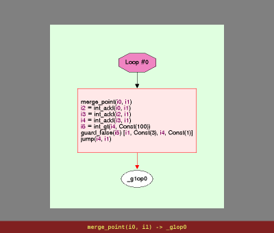
It's entering JIT, doing some primitive operations for bytecode dispatching and repeating the loop. Note that at the end of the interpreted loop (not to be confused with the interpreter loop), we see int_sub [3, 3] which resets the bytecode position to the beginning. At this time JIT (instructed by can_enter_jit hint) notices that all green variables are the same (here only i), hence we can compile the efficient loop from this point.

The loop contains 3 additions and a check (for i < 100), exactly the same as our interpreted program would do, but completely without interpretation overhead!

As you might have noticed, there is no assembler involved so far. All of this instruction execution is done directly, in pure python. In fact, the code for executing instructions is located in jit/backend/llgraph which directly interprets instructions. This is by far simpler (and easier to debug) than x86 assembler.

And this is basically it: the very simple interpreter and a jit for it. Of course we actually can generate assembler for that. Also the missing piece is optimizing the generated graphs. While for this example, by removing the interpretetation overhead, we're done, with more complex examples it's important to further optimize traces. Hopefully this and how we actually generate assembler will be topics for next blog posts.

Cheers,
fijal